Heterogeneous Treatment Effects at Netflix

Learn more about our work on HTEs and experimentation at CODE@MIT 2025!

At Netflix, we invest heavily in understanding the causal impact of our actions. Often, this impact is heterogeneous: a software update may affect legacy firmware differently than new firmware, a homepage redesign might cause more signups in one country than another, and some members may prefer push notifications whereas others may prefer email. Capturing this heterogeneity is valuable for many reasons, from catching regressions to delivering a member experience that feels personalized.

Over time, we’ve honed our ability to detect, measure, and act on heterogeneous treatment effects (HTEs). In this post, we’ll share five case studies on how HTEs influence all phases of product experimentation and innovation at Netflix.

Discovery: finding unforeseen causal effects on subpopulations. This detection is especially important for technical changes like app updates, which affect hundreds of different device types. With so many segments, false discovery is a major concern. We’ll explain how we control the false discovery rate while surfacing genuinely problematic interactions.
Hypothesis Generation: exploring potential levers for improving the Netflix experience. One valuable tool here is Observational Causal Inference (OCI), which we use to generate early insights for further testing in experiments. We’ll share how our OCI platform enables rapid segmentation and exploration of HTEs.
Deciding Experiments: choosing which A/B-tested experiences should be rolled out. HTEs are often critical to understanding the total effect of a new experience on long-term member satisfaction. We’ll explain how we incorporate such heterogeneity when making decisions.
Estimating Annualized Impacts: understanding the long-term impact of rolled-out experiences on core business metrics. This facilitates standardized comparisons across tests and/or segments, which in turn enables opportunity sizing and resource allocation optimization. We’ll demonstrate how we quantify the annualized impact of our deployments more accurately using HTEs.
Policy Learning and Personalization: using learned HTEs to design personalized experiences. Once we find evidence of heterogeneity in an A/B test, the next question is often whether it is worth the cost of further personalizing the experience. We’ll explain how we estimate the incremental value of personalization over productizing the “global winner” (the arm with the largest average treatment effect).

We’re especially pleased to be presenting two of these case studies at this week’s Conference on Digital Experimentation at MIT (CODE@MIT):

Estimating Annualized Impacts in the Parallel Session A on long-term treatment effects on Friday, November 14 at 10:40am.
Policy Learning and Personalization in the Parallel Session I on policy learning on Friday, November 14 at 2:50pm.

Discovery

Scott Seyfarth

The Netflix apps run on millions of TVs, cell phones, tablets, and other devices. When we update them with new features or bug fixes, we want to ensure that every update works as expected. We use A/B testing to help discover whether any devices respond poorly to the update. But by the time we share the update with our members in an A/B test, we’ve already tested it extensively and are confident it works well. When problems do arise, they usually only affect a few device types. How do we find these needles in a haystack?

One approach would be to use a frequentist hypothesis test to decide if there is a significant difference between the treatment and control cells in the number of crashes per device type, with an adjustment such as the Bonferroni correction. This guarantees that the overall probability of one or more significant tests when the null is true is no more than the nominal rate (usually 1 in 20).

In our context — with frequent updates and thousands of device types — this guarantee is not very useful. Most app updates do not cause problems on any device, and false alerts on 1 in 20 of these updates would quickly erode trust. Rather than guarantee a false alert on every 20th update, we prefer to guarantee that any alerts have a low probability of being false. This is a guarantee about the false discovery rate (Benjamini & Hochberg 1995) that can also be understood as the Bayesian posterior probability of the null hypothesis (Efron et al. 2001, Efron 2005).

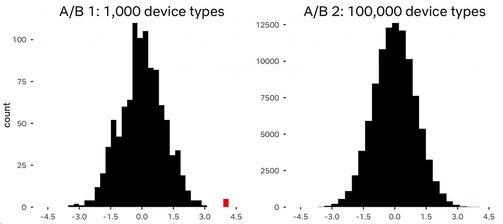
To illustrate this idea, we simulated the distribution of z-scores in two different A/B tests. The first A/B test includes 1,000 unique device types (left), while the second A/B test includes 100,000 device types (right). Most device types will run the update smoothly, so the z-scores will follow a standard normal distribution. A handful of devices may respond poorly, and thus have large z-scores that follow an alternative distribution. In both A/B tests, we observe five device types that have a z-score around 4, shown in red in both panels below. Are these five device types drawn from the null-hypothesis standard normal distribution, or from an alternative?

In both A/B tests, a z-score of 4 is statistically significant. Nevertheless, when visualizing the distribution of test statistics, most folks will have the intuition that with 1,000 total device types, the five devices with z = 4 are outliers. But when 100,000 device types are tested, it seems much more likely that the five red device types are still part of the null distribution. With 100,000 samples, the five at z = 4 fall within the bell curve of the null.

Visualizing the empirical distribution of test statistics is often sufficient for our software developers to recognize outliers that may be problematic: z-scores that fall outside the bell curve are worth investigating. Using Bayes’ theorem, this intuition can also be formalized as the posterior probability of the null hypothesis given an observation with z = 4, or what Efron et al. 2001 call the local false discovery rate. Our A/B testing platform estimates this probability and reports it to developers for each device type, which alerts them to genuine problems and helps them avoid investigating false positives in a setting where true positives are rare.

Hypothesis Generation and Member Understanding

Adrien Alexandre

Data Scientists at Netflix work on a huge variety of problems, from safeguarding app updates to improving the holistic member experience. A focus of our Member Data Science team is how to measure long-term satisfaction of our members. While our top-line metric for long-term satisfaction is subscriber retention, we necessarily rely on more sensitive metrics to inform product launch decisions, while still maintaining confidence in our progress towards this North Star.

When building such proxies, we rely heavily on Observational Causal Inference (OCI) to infer relationships between metrics (e.g., establishing the causal relationship between viewing and retention). It’s likely that these causal relationships differ across subpopulations. For example, while viewing is important to all members, it’s especially critical for us to help new members find titles to stream and enjoy. By breaking down these HTEs, we’re able to construct proxy metrics that capture nuances in our customer base, such that our predictions of long-term impact are more accurate; and to inform innovations that respond to the diverse needs of our member base.

To facilitate rapid exploration of these causal questions, HTEs are a core part of our internal OCI platform at Netflix. The backbone of this platform is the Augmented Inverse Propensity Weighting (AIPW) estimator. AIPW combines an outcome regression and a propensity model to form a doubly robust score. Specifically, we construct a “pseudo-outcome” for each unit and treatment level:

which leverages the conditional outcome model m and propensity score model e given a realized outcome Y, pretreatment covariates X, and treatment T.

Since we construct these pseudo-outcomes for all units and treatments, it is easy to compute Conditional Average Treatment Effects (CATEs) simply by averaging the pseudo-outcomes in subgroups of interest (for example, new members or grouping by region).

Most of the effort involved in building these pseudo-outcomes is in producing the outcome and propensity models, so this approach helps us to strike the right balance between 1) establishing actionable insights into subgroup differences and 2) optimizing the platform’s compute and memory footprint, improving performance.

Deciding Experiments

Carlos Velasco Rivera and Colin Gray

For many years, Netflix has been synonymous with streaming. Today, we are expanding into new domains, from games to live sports to Netflix House. With these increased business offerings comes potential tradeoffs. For example, what if a recommendation algo change causes users to play more games but watch fewer movies? What if another change causes users to watch more movies but fewer TV shows? We’ve learned that these tradeoffs vary meaningfully among different types of users, and we use HTEs to help inform product innovation when they arise.

To balance these tradeoffs, we would ideally rely on North Star metrics, such as subscriber retention, directly. However, these metrics are often slow-moving and too insensitive to target in most experiments. Instead, we rely on proxy metrics, which are correlated with the North Star but much more precise. Using tools like OCI to explore candidate metrics and historical meta-analysis to narrow down on the strongest signals, we estimate the causal impact of different proxy metrics on the North Star. This gives us an “exchange rate” that helps us to determine whether a given tradeoff between these metrics results in an expected gain to the north star or not.

We supercharge this idea using HTEs. Usually, the causal impact of a proxy metric varies widely across subgroups. For example, some members especially value playing games, others especially value movies, and still others might prioritize watching their favorite TV shows week over week. Using group-specific exchange rates helps us make better decisions that reflect the heterogeneous preferences in our member base, while still blending these into a unified estimate to guide decisions.

Our framework is highly extensible. For example, suppose we have two subgroups and two metrics X and Z. Using a variety of causal methods including OCI and meta-analysis, we estimate the HTEs of each metric in each subgroup on our North Star. Lastly, we estimate a blended metric that helps us decide whether a treatment is beneficial on balance for that subgroup.

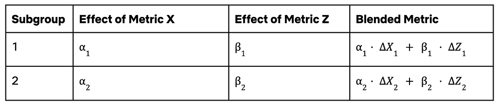
We can easily extend this framework to cover more proxies by expanding the table horizontally and more subgroups by expanding the table vertically. Revealing these differences helps us to make better decisions that are sensitive to the heterogeneity of our member base and oriented towards long-term success.

Estimating Annualized Impacts

Tomoya Sasaki, Simon Ejdemyr, and Mihir Tendulkar

Tomoya will present on this topic at CODE@MIT on Friday, November 14 at 10:40am.

Once experiments have been decided and features launched, we need to translate their short‑term experimental results into annualized, population‑level business impacts. Doing so has two benefits: (1) dollar-based cost-benefit analysis, which allows teams to weigh expected financial returns against implementation and operational costs; and (2) consistent cumulative effects tracking across experimentation programs, even when those programs target different populations or metrics. This is especially important when HTEs reveal differences across segments and/or markets, which may have different growth strategies and trajectories.

We developed an automated tool to estimate the annualized impact of a treatment inclusive of current and future member cohorts. Under this framework, the first month cohort contributes to revenue for 12 months, the second month cohort for 11 months, …, and the twelfth month cohort for 1 month.

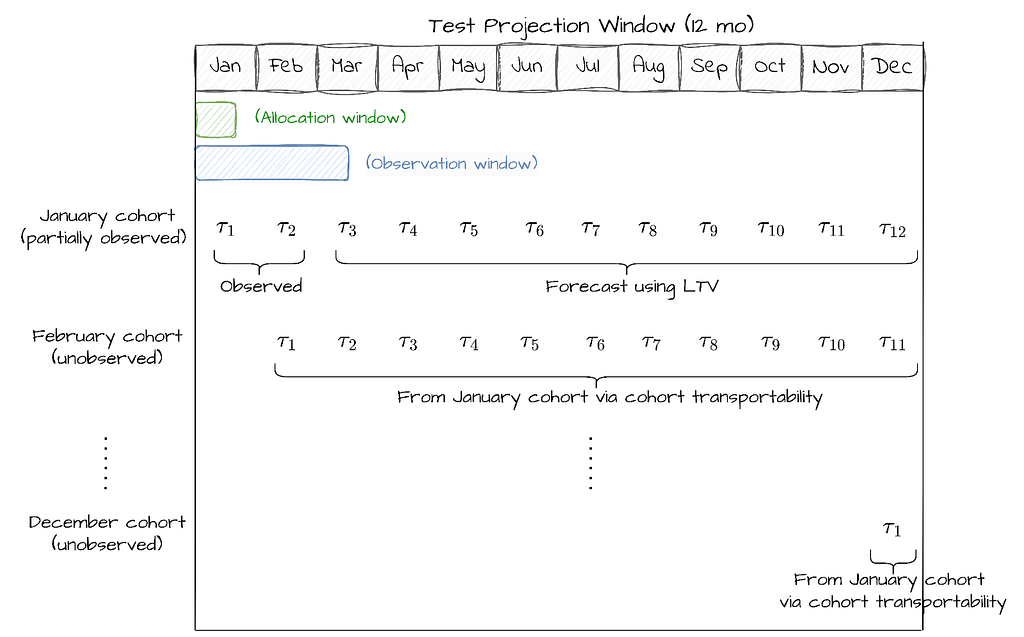
Let’s break down the methodology using a simple example. Suppose we allocate users for one month (January) in an A/B test and monitor outcomes for the next billing period. Thus, we observe one monthly cohort and its treatment effects in the two billing periods. To estimate annualized impact, we rely on the observed treatment effects for month 1 and 2 (1 and 2) , observed traffic, and three unobserved quantities: (1) the treatment effects for the remaining 10 billing periods of the first cohort, (2) the traffic for the subsequent 11 cohorts, and (3) and treatment effects for those subsequent cohorts.

Our tool estimates both quantities using the following approach. First, to obtain the treatment effects for the unobserved billing periods of the observed cohort, we model future potential outcomes via surrogacy based on a Lifetime Value (LTV) prediction model. Second, we apply a transportability assumption that stipulates that each subsequent cohort’s period-by-period treatment effects match those for the first cohort. Lastly, we sum these effects to obtain the annualized impact. Our tool enables analysts to model population growth or decay as needed, accommodating scenarios where growth or seasonality is expected.

To strengthen our assumptions and increase accuracy, we often find it helpful to apply this algorithm on a per-segment basis — using HTEs along with segment-specific growth projections. This approach allows us to produce more granular estimates and facilitates comparisons between experimentation programs that target different populations.

Policy Learning and Personalization

Shusei Eshima and Sambhav Jain

Shusei will present on this topic at CODE@MIT on Friday, November 14 at 2:50pm.

Last but not least, we also use HTEs to help guide personalization: providing a Netflix experience that feels relevant and specific to every member. These learnings are built on top of the many experiments we run to learn which experiences best serve our members.

These experiments often have treatment arms (or “cells”) that perform comparably well. For example, in an experiment with four treatment cells, we might observe that Cells 2 and 4 perform comparably well compared to the control. Should we select Cell 4 simply because it appears to be slightly better than Cell 2?

Scrutinizing the experiment results, we may find segments for which Cell 2 drives a better outcome than Cell 4. We call this a meaningful HTE because it means that a personalized treatment policy can drive better outcomes than simply launching the global winner. To identify meaningful HTEs, we must look at segments both (1) across cells (to check if a particular segment might see an even more positive outcome in the primary metric if exposed to a different cell) and (2) within the global winner (to check if a particular segment has a negative reaction even if the cell is positive overall).

In our effort to find meaningful HTEs scalably, we encounter three key challenges: (1) defining segments, (2) deriving personalized treatment rules, and (3) ensuring these rules are explainable, which is critical to informing product development and innovation.

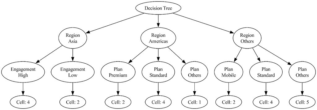
To address these challenges, we leverage the policy tree literature (Zhou et al., 2023). We also make two key innovations to suit our needs. First, we develop an m-ary tree search algorithm for categorical variables, rather than the traditional binary tree. This approach enables us to capture more nuanced member segments. Second, we implement a scalable policy learning algorithm capable of analyzing data from millions of members in our experiments.

Our method has two steps. First, as in our OCI platform, we calculate the doubly robust score to estimate counterfactual outcomes for each member. Second, we construct a decision tree that simultaneously optimizes this score and identifies segments that maximize our outcome metric. The structure of the decision tree makes the resulting segments and personalization rules interpretable, allowing us to communicate our insights to stakeholders.

Here are two figures that illustrate our approach. First, we show an example of an m-ary tree, where the variables “region” and “plan” branch into three child nodes.

Second, we demonstrate the business impact of personalization. We compare binary and m-ary trees at various depths by training the policy on a training dataset and evaluating it on a test dataset. The leftmost estimate corresponds to the global winner, which assigns the single best cell to all members. Using an m-ary tree yields a statistically significant improvement over the global winner, whereas a binary tree does not.

Evidence of this kind clearly demonstrates the business impact of personalization, helping us to make better decisions about when a treatment is worth personalizing and when it is sufficient to roll out the global winner.

Conclusion

Taken together, these case studies show how we use HTEs across the full lifecycle of product innovation — from catching regressions before they ship to deciding launches and ultimately powering personalization. These pieces form a modular toolkit that connects together in practical ways, for example:

Exploration feeds into decision-making. OCI helps teams quickly explore candidate proxy metrics and their heterogeneous impacts on North Star, which can then be refined via historical meta-analysis into decision metrics.
Annualized estimates guide personalization. Our annualized-impact models provide a consistent, dollar-based view of long-term effects. When applied to policy learning, they help us assess when a global winner is sufficient versus when a personalized policy creates more value.

This modularity reflects our highly aligned and loosely coupled culture. Although different verticals build components to address local problems, we strive to combine these elements into a coherent system for informing decision-making and personalization at scale.

Interested to learn more and attending CODE@MIT? Check out our booth to meet Netflix Data Scientists, view recent research publications, and check out job opportunities!

By Scott Seyfarth, Adrien Alexandre, Carlos Velasco Rivera, Colin Gray, Tomoya Sasaki, Shusei Eshima, Sambhav Jain, Simon Ejdemyr, Mihir Tendulkar, Matthew Wardrop, and Winston Chou