How and Why Netflix Built a Real-Time Distributed Graph: Part 2 — Building a Scalable Storage Layer

This is the second entry of a multi-part blog series describing how we built a Real-Time Distributed Graph (RDG). In Part 1, we discussed the motivation for creating the RDG and the architecture of the data processing pipeline that populates it. In Part 2, we’ll explore how we designed the storage layer to handle billions of nodes and edges while maintaining single-digit millisecond latencies.

Introduction

In Part 1 of this series, we explained why Netflix needed a Real-Time Distributed Graph (RDG) and how we built the ingestion and processing pipeline using Apache Flink to transform streaming events into graph primitives. Now comes the following critical question: once we’ve created billions of nodes and edges from member interactions, how do we actually store them?

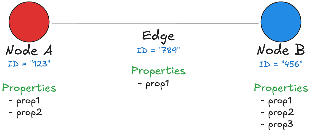
The Graph Data Model

Before diving into storage technology, let’s clarify what we’re actually storing.

The RDG is a property graph consisting of:

Nodes: Entities including member accounts, titles (such as shows/movies), devices, and games. Each node has a unique identifier and a set of properties containing additional metadata.
Edges: Relationships between nodes, such as “started watching,” “logged in from,” or “plays.” Edges also have unique identifiers and properties, such as timestamps.

Let’s revisit our example from Part 1.

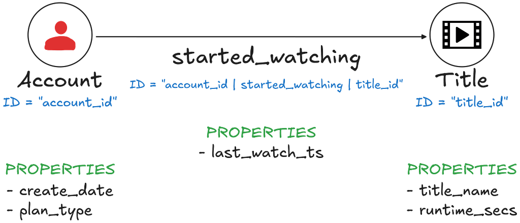
When a member watches Stranger Things, we might create:

An “account” node (with properties like creation_date and plan_type)
A “title” node (with properties like title_name and runtime_secs)
A “started watching” edge connecting the nodes above (with properties like last_watch_timestamp)

This simple abstraction allows us to represent incredibly complex member journeys across the Netflix ecosystem. But how do we efficiently store and query this graph structure at scale?

Graph Databases

The storage layer is the backbone of the RDG. It needs to efficiently store billions of nodes and hundreds of billions of edges while supporting both heavy read and write workloads with low latency.

In evaluating different storage options, we explored traditional graph datastores like Neo4J and AWS Neptune. While they do provide feature-rich capabilities around things like native-graph query support and data models to represent different types of graphs, they also pose a mix of scalability, workload, and ecosystem challenges.

Scale and performance limitations

Native graph databases, while excellent for exploring relationships, struggle to scale horizontally for large, real-time datasets. Their performance typically degrades with increased node and edge count or query depth (i.e., more hops). In our own early evaluations, Neo4j, for example, performed well for millions of records but became inefficient for hundreds of millions due to high memory requirements and limited distributed capabilities. AWS Neptune has similar limitations due to its single-writer, multiple-reader architecture, which presents bottlenecks when ingesting large data volumes in real-time, especially when spanning multiple regions. These limitations made them unsuitable for workloads demanding low-latency access, particularly in distributed systems where data sharding is required.

Workload complexity

Traditional graph database solutions often present significant challenges when faced with the demands of Netflix’s high-volume, real-time data environment. These systems are not inherently designed or optimized for the continuous, high-throughput event streaming and real-time data ingestion workloads that are critical to our operations, and they frequently struggle with query patterns that involve full dataset scans, property-based filtering, and indexing. This made it clear that we needed an alternative capable of handling our internet-scale data.

Internal support

At Netflix, we have extensive internal platform support for relational and document databases, compared to graph databases. Consequently, non-graph databases are also easier for us to operate. As a result, we found it simpler to emulate graph-like relationships in existing data storage systems rather than adopting specialized graph infrastructure.

Due to the reasons mentioned above, we ultimately decided that the options we evaluated wouldn’t meet our requirements at Netflix’s scale. Therefore, we turned instead to an internal platform specifically designed for this type of challenge: the Data Gateway Platform. More specifically, its Key-Value Data Abstraction Layer (KVDAL).

Why KVDAL?

The Data Gateway Platform at Netflix provides several Data Abstraction Layers (DALs) that sit between applications and databases. These DALs support different data access patterns while delivering high availability, tunable consistency, and low latency, all without the operational overhead of managing underlying storage infrastructure directly.

For the RDG, we chose KVDAL as our primary storage solution. KVDAL is built on top of Apache Cassandra and provides a two-level map architecture that proved to be a perfect fit for graph data.

The KVDAL Data Model

KVDAL organizes data into records that are uniquely identified by a record_id. Each record can contain one or more sorted items, where an item is simply a key-value pair. This structure looks like the following:

To query KVDAL, you:

First, look up a specific record by its record_id
And then (optionally) filter and retrieve only the subset of items you’re interested in by their keys

This two-level architecture gives us both efficient point lookups and the flexibility to retrieve related data with minimal overhead.

Mapping Graphs to Key-Value Storage

The elegance of KVDAL for graph storage becomes clear when we examine how nodes and edges are mapped to records.

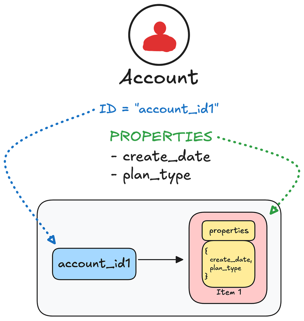
Storing Nodes

When storing nodes:

The node’s unique identifier becomes the record_id
All properties for that node are stored as a single item within the record

For example, an account node might look like:

Storing Edges as Adjacency Lists

When storing edges, we rely heavily on adjacency lists, which are a way of representing a graph where, for every node in the graph, we have a list that contains the nodes that are adjacent to it.

For our use case, this means that:

The record_id represents the “from” node of the edge
While the items within that record represent all the “to” nodes that the “from” node connects to
Just like nodes, edges can also store properties within an item.

For example, if an account has watched multiple titles, the adjacency list might look like the following:

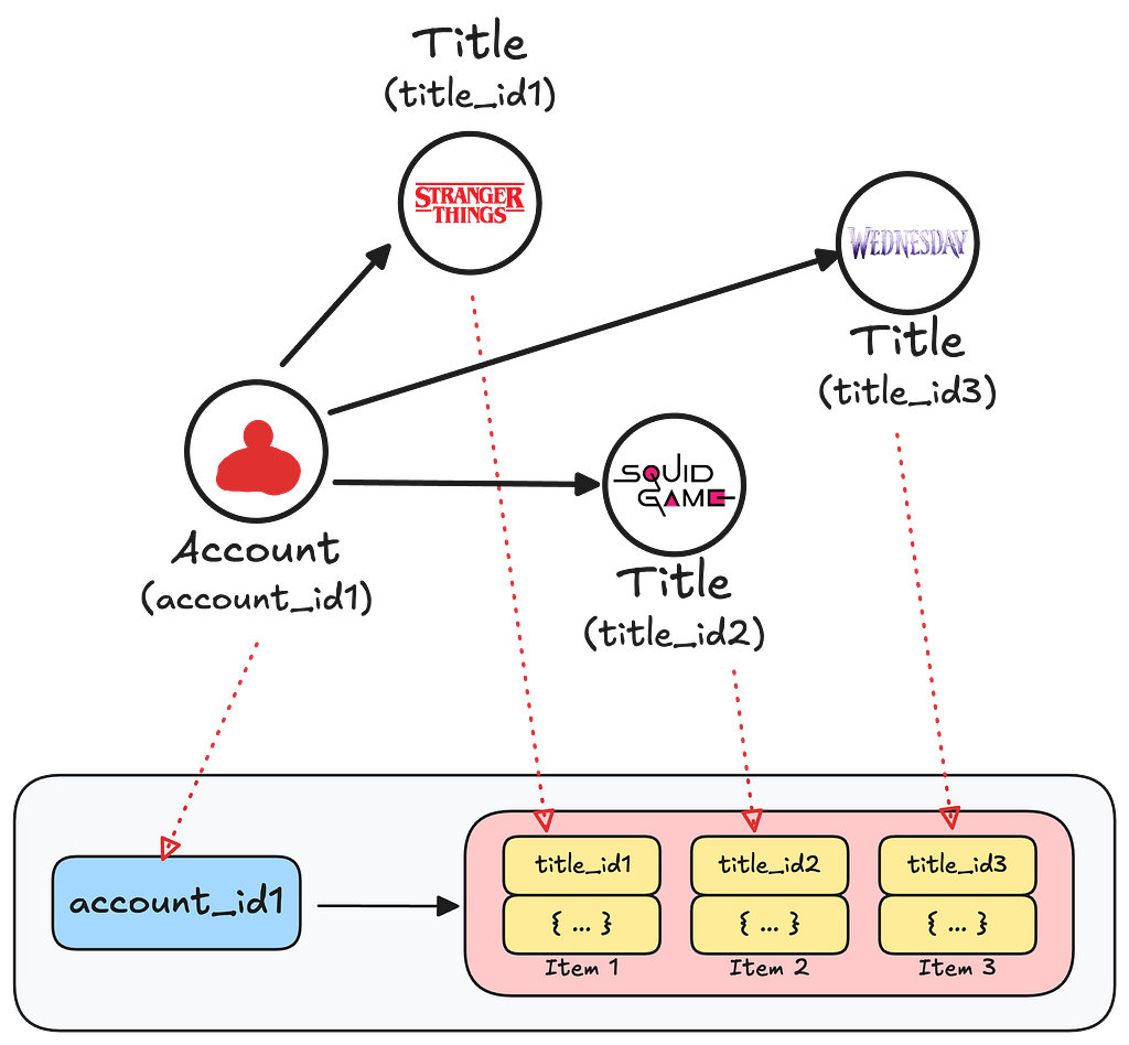
This adjacency list format is vital for graph traversals. When we need to find all titles a member has watched, we can retrieve the entire record with a single KVDAL lookup. But we can also filter by specific titles using KVDAL’s key filtering, avoiding the need to fetch and deserialize unnecessary data.

Data Lifecycle

The lifecycle of the node and edge data stored in RDG is relatively straightforward. In Part 1, we covered how we constantly ingest real-time event streams that are converted into node and edge objects before being stored in the graph. Whenever we ingest new nodes or edges that we haven’t seen before, KVDAL simply creates new records for them. In cases where an edge exists with an existing “from” node but a new “to” node, we would create a new item within the existing KVDAL record. There are other times when we might ingest the same node or edge multiple times. When this happens, we simply overwrite the existing values within KVDAL, which means overwriting the entire record for nodes or the corresponding items for edges. This gives us the ability to continuously update the nodes and edges in the graph with the most recent property values, which is essential for keeping specific properties (e.g., timestamps) up to date.

KVDAL can also automatically expire data after a specific period of time on a per-namespace, per-record, or per-item basis. This not only provides us with a lot of flexibility and fine-grained control over how we expire data from the graph on a per-node-type and per-edge-type basis, but it also allows us to create limits on how large different parts of the graph can get.

Namespaces: The key to flexibility and scale

One of the most powerful KVDAL features that we leveraged for RDG is the concept of namespaces. A namespace is similar to a table in a traditional database. It’s a logical grouping of records that defines where data is physically stored while abstracting away details of the underlying storage system.

This means that you could start with a KVDAL setup where all of your namespaces are backed by the same Cassandra cluster.

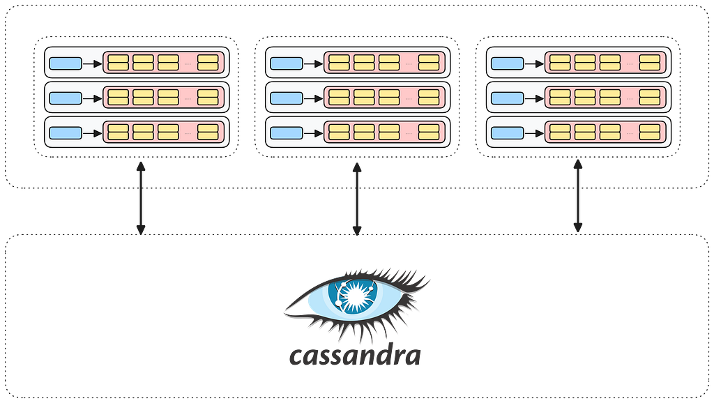
However, suppose one of these namespaces needs to store more data than the others, or it begins to receive a disproportionately larger amount of traffic compared to the others. In that case, we can simply move it to its own cluster as a way to isolate it from the rest of the setup, allowing it to be managed and scaled independently.

Similarly, if your namespaces have different requirements around performance and scalability, we can further customize them by moving each namespace to its own dedicated storage setup in order to meet those needs.

Because of this flexibility, KVDAL can scale to support trillions of records per namespace with single-digit millisecond access latencies.

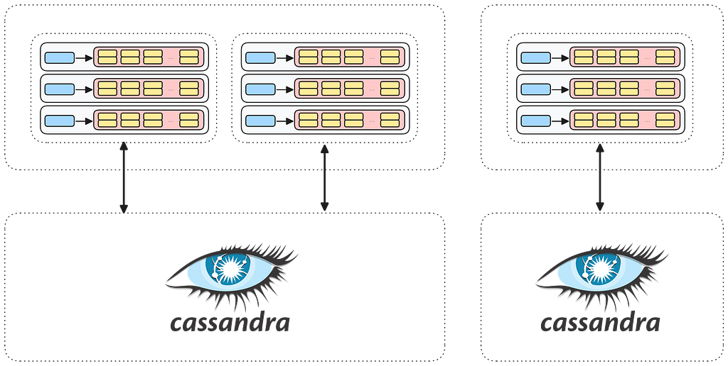
One namespace per node and edge type

For the RDG, we provision a separate namespace for every node type and edge type in the graph. This might seem like overkill at first, but it provides us with a lot of benefits, including:

Independent Scaling: Different parts of the graph have vastly different data volumes and access patterns. By isolating each entity type into its own namespace, we can scale and tune each one independently from the others.

Flexible Storage Backends: Namespaces can be backed by different Cassandra clusters or entirely different storage technologies. For example:

Low-latency data might use Cassandra with EVCache for caching
Average throughput data with more lenient requirements around latency might use a single Cassandra cluster to host multiple namespaces
Extremely high-throughput data might use dedicated Cassandra clusters per namespace

Operational Isolation: If one namespace experiences issues or needs maintenance, it doesn’t impact the rest of the graph. This isolation is critical for maintaining system reliability at scale.

Flexibility when adding new entity types

This namespace model also makes it straightforward to extend the RDG with new types of nodes and edges. When we need to support a new use case, say, adding support for tracking member interactions with live events, we would simply:

Define the new node and edge types in our data model
Provision new KVDAL namespaces for them
Update our Flink jobs to populate these namespaces (see Part 1 for details)
Deploy without impacting existing functionality

This flexibility was a key design goal from the beginning. We wanted to ensure the RDG could support unknown future use cases without significant re-architectural efforts.

By the numbers

So how well does this architecture actually perform in practice?

Currently, our graph comprises over 8 billion nodes and more than 150 billion edges across all the different use cases we support. In terms of throughput, we have achieved concurrent reads and writes at sustained rates of approximately 2 million reads/sec and 6 million writes/sec across all nodes and edges in the graph.

To support this, we currently operate a KVDAL cluster that consists of approximately 27 different namespaces, backed by around 12 Cassandra clusters across 2,400 EC2 instances.

These numbers represent one of the larger Cassandra deployments at Netflix. However, it’s important to note that the numbers listed above aren’t hard limits. Every component in our architecture can scale linearly. As the graph continues to grow, we can add more namespaces, clusters, and instances as needed.

Looking Ahead

Building the RDG’s storage layer required significant engineering investment, and not everything was smooth sailing. Throughout its development, we encountered scaling challenges with various parts of the infrastructure and had to rework the data model several times. Through extensive iteration and performance tuning, we arrived at a solution that met our needs. These challenges also taught us valuable lessons about operating graph systems at scale.

Despite the bumps along the way, the RDG has delivered exceptional flexibility, scalability, and reliability. We were fortunate to build on the shoulders of giants by leveraging KVDAL’s namespace model and the battle-tested reliability of Cassandra. Thanks to this robust infrastructure and unwavering support from our platform teams, we created a foundation that can evolve alongside Netflix’s business needs.

Furthermore, our learnings benefited not only the RDG. In fact, they uncovered opportunities to generalize our solutions and, to that end, we partnered with our online datastores team to develop a broader graph abstraction platform that can support other graph use cases across Netflix. Stay tuned for a separate blog post that will provide more details about this exciting work.

—

Thanks for reading Part 2 of the RDG blog series. Stay tuned for Part 3, where we’ll dive into the serving layer and explore how we make this massive graph accessible for use cases across Netflix.